thought:
If the variable W is used to represent n words arranged in sequence in a text, ie W = W1W2...Wn, then the task of the statistical language model is to give the probability P(W) of the sequence of arbitrary words W appearing in the text. Using the product of the probability formula, P(W) can be expanded to: P(W) = P(w1)P(w2|w1)P(w3| w1 w2)...P(wn|w1 w2...wn-1), no It is easy to see that in order to predict the probability of occurrence of the word Wn, the probability of occurrence of all words in front of it must be known. From a computational point of view, this is too complicated. If the probability of occurrence of any word Wi is only related to the N-1 words in front of it, the problem can be greatly simplified. The language model at this time is called the N-gram model, that is, P(W) = P(w1)P(w2|w1)P(w3| w1 w2)...P(wi|wi-N+1...wi -1)... The actual use is usually a binary model (bi-gram) or a tri-gram of N=2 or N=3. Taking the ternary model as an example, it is approximated that the probability of occurrence of the arbitrary word Wi is only related to the first two words immediately following it. It is important that these probability parameters are all evaluable through a large-scale corpus. For example, the ternary probability has P(wi|wi-2wi-1) ≈ count(wi-2 wi-1... wi) / count(wi-2 wi-1) where count(...) represents a specific word sequence throughout The cumulative number of occurrences in the corpus. The statistical language model is a bit like the method of weather forecasting. The large-scale corpus used to estimate the probability parameters is a meteorological record accumulated over the years. The use of the ternary model for weather forecasting is like predicting today's weather based on the weather conditions of the previous two days. The weather forecast is certainly not 100% correct. This is also a feature of the probability and statistics method. (Excerpt from Huang Changning's paper "What is the mainstream technology of Chinese information processing?")
Condition: The model is based on the assumption that the occurrence of the nth word is only related to the previous N-1 words, and is not related to any other words. The probability of the whole sentence is the product of the probability of occurrence of each word. These probabilities can be obtained by counting the number of simultaneous occurrences of N words directly from the corpus. Commonly used are binary Bi-Gram and ternary Tri-Gram.
problem:
Although we know that the larger the n is, the stronger the binding force is, the difficulty of large n statistics is difficult due to the limitation of computer capacity and speed and the sparse data.
Second, Markov model and hidden Markov model
Thought: The Markov model is actually a finite state machine. There is a transition probability between the two states. In the hidden Markov model, the state is not visible. We can only see the output sequence, that is, each state transition will throw an observation. Value; when we observe the observation sequence, we need to find the best state sequence. Hidden Markov Model is a parametric model used to describe the statistical properties of stochastic processes. It is a double stochastic process consisting of two parts: Markov chain and general stochastic process. The Markov chain is used to describe the state transition and is described by the transition probability. A general stochastic process is used to describe the relationship between a state and an observed sequence, and is described by the observed value probability. Therefore, the hidden Markov model can be regarded as a finite state automaton capable of randomly performing state transition and outputting symbols. It models the stochastic generation process by defining the joint probability of the observed sequence and the state sequence. Each observation sequence can be regarded as being generated by a state transition sequence. The state transition process starts by randomly selecting an initial state according to the initial state probability distribution, outputs an observation value, and then randomly shifts to the next state according to the state transition probability matrix until Arriving at a pre-specified end state, each state will randomly output an element of the observation sequence according to the output probability matrix.
An HMM has five components, usually written as a five-tuple {S, K, π, A, B}, sometimes abbreviated as a triple {π , A, B}, where: 1S is the state set of the model The model has a total of N states, denoted as S={s1, s2, ⋯, sN}; 2K is a set of state output symbols in the model, the number of symbols is M, and the symbol set is recorded as K={k1, k2, ⋯, kM }; 3 is the initial state probability distribution, denoted as = { 1, 2, ⋯, N}, where i is the probability of state Si as the initial state; 4A is the state transition probability matrix, denoted as A = {aij}, 1 ≤ i ≤ N, 1 ≤ j ≤ N. Where aij is the probability of transitioning from state Si to state Sj; 5B is the symbol output probability matrix, denoted as B={bik}, 1≤i≤N, 1≤k≤M. Where bik is the probability that state Si outputs Vk. To solve the practical problem with HMM, we first need to solve the following three basic problems: 1. Given an observation sequence O=O1O2⋯OT and the model {π, A, B}, how to calculate the probability P(O|λ) efficiently, That is, the probability of observing the sequence O in the case of a given model; 2 given an observation sequence O = O1O2 ⋯ OT and the model { π, A, B}, how to quickly select the "optimal" state in a certain sense The sequence Q = q1q2 ⋯ qT, so that the state sequence "best interpretation" of the observation sequence; 3 given an observation sequence O = O1O2 ⋯ OT, and possible model space, how to estimate the model parameters, that is, how to adjust The parameters of the model {π, A, B} are such that P(O|λ) is the largest.
problem:
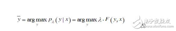
There are two hypotheses in the hidden horse model: the output independence hypothesis and the Markov assumption. Among them, the output independence hypothesis requires that the sequence data is strictly independent of each other to ensure the correctness of the derivation, and in fact most of the sequence data cannot be represented as a series of independent events. Third, the maximum entropy model The principle of maximum entropy was originally a very important principle in thermodynamics, and was later widely used in natural language processing. The basic principle is simple: model all known facts and make no assumptions about the unknown. That is to say, such a statistical probability model is selected during modeling, and the probability model with the largest entropy is selected in the model satisfying the constraint. If the part-of-speech tagging or other natural language processing tasks are regarded as a stochastic process, the maximum entropy model is to select the most uniform distribution from all the eligible distributions, and the entropy value is the largest. To solve the maximum entropy model, the Lagrangian multiplier method can be used, and its calculation formula is:
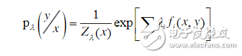
For the normalization factor,  Is the weight of the corresponding feature,
  Represents a feature. The magnitude of the influence of each feature on part of speech selection by feature weight
  Decide, and these weights are automatically obtained by GIS or IIS learning algorithms.
Principle: The main idea of ​​SVM can be summarized as two points: (1) It is analyzed for linear separable cases. For linear indivisible cases, the non-separable samples of low-dimensional input space are transformed into non-separated samples by using nonlinear mapping algorithms. The high-dimensional feature space makes it linearly separable, which makes it possible to linearly analyze the nonlinear characteristics of the sample using a linear algorithm in high-dimensional feature space. (2) It constructs the optimality in the feature space based on the theory of structural risk minimization. The hyperplane is segmented such that the learner is globally optimized and the expected risk across the sample space satisfies a certain upper bound with a certain probability. The goal of SVM is to construct an objective function to distinguish the two types of patterns as much as possible according to the principle of structural risk minimization. It is usually divided into two categories: (1) linear separability; (2) linear inseparable .
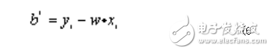
Linearly separable cases In the case of linear separability, there is a hyperplane that completely separates the training samples, which can be described as: w · x + b = 0 (1) where "·" is the dot product, w is an n-dimensional vector and b is an offset.
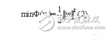
The optimal hyperplane is such a plane that maximizes the distance between the vector and the hyperplane where each type of data is closest to the hyperplane.
The optimal hyperplane can be obtained by solving the following quadratic optimization problem:
Meet the constraints: 
In the case of a particularly large number of features, this quadratic programming problem can be transformed into its dual problem:
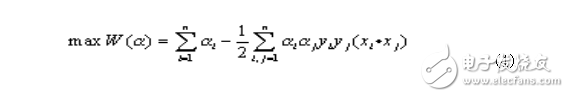
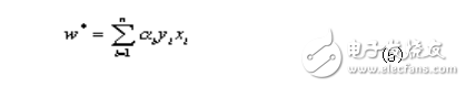
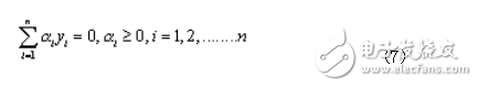
Meet the constraints:
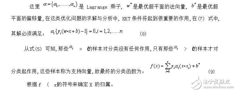
Linear indivisible case For linear indivisible cases, the sample X can be mapped to a high-dimensional feature space H, and the original space function is used in this space to implement the inner product operation, thus transforming the nonlinear problem into another space. Linear problem to get the attribution of a sample. According to the relevant theory of the functional, as long as a kernel function satisfies the Mercer condition, it corresponds to the inner product in a certain space, so this linear indivisible classification can be realized by using an appropriate inner product function on the optimal classification surface. problem. The objective function at this time is: Figure XII
Features:
In a nutshell, the support vector machine first transforms the input space into another high-dimensional space by the nonlinear transformation defined by the inner product function, and finds the optimal classification surface in this space. The SVM classification function is similar in form to a neural network. The output is a linear combination of intermediate nodes. Each intermediate node corresponds to an inner product of an input sample and a support vector, so it is also called a support vector network. Characteristics of SVM method: 1 Nonlinear mapping is the theoretical basis of SVM method. SVM uses inner product kernel function instead of nonlinear mapping to high-dimensional space; 2 optimal hyperplane for feature space partitioning is the target of SVM, maximizing classification The marginal idea is the core of the SVM method; 3 The support vector is the training result of the SVM, and the support vector plays a decisive role in the SVM classification decision. SVM is a novel small sample learning method with a solid theoretical foundation. It basically does not involve probability measures and laws of large numbers, so it is different from existing statistical methods. In essence, it avoids the traditional process from induction to deduction, and achieves efficient "transduction reasoning" from training samples to forecast samples, greatly simplifying the problems of general classification and regression. The final decision function of the SVM is determined by only a few support vectors. The computational complexity depends on the number of support vectors, not the dimensions of the sample space, which in some sense avoids the "dimension disaster." A few support vectors determine the final result, which not only helps us to grasp the key samples, "cull" a large number of redundant samples, but also destined that the method is not only simple, but also has a good "robust". This "robustness" is mainly reflected in:
1 Adding and deleting non-support vector samples have no effect on the model; 2 Support vector sample sets have certain robustness; 3 In some successful applications, the SVM method is not sensitive to kernel selection.
4. Conditional Random Field Principle: Conditional Random Fields (CRFs) is a statistical-based sequence marker recognition model first proposed by John Lafferty et al. in 2001. It is an undirected graph model that calculates the conditional probability on a given node's output value for a given node input value, with the training goal of maximizing the conditional probability. Linear chains are one of the specific graph structures commonly found in CRFs, which are sequentially linked by specified output nodes. A linear chain corresponds to a finite state machine and can be used to solve the labeling problem of sequence data. In most cases, CRFs refer to linear CRFs. The data sequence to be labeled is represented by x = (x1, x2, ..., xn), and y = (y1, y2, ..., yn) represents the corresponding result sequence. For example, for Chinese part-of-speech tagging tasks, x can represent a Chinese sentence x=(Shanghai, Pudong, development, and, legal, construction, synchronization), and y means the part-of-speech sequence y=(NR, NR, for each word in the sentence. NN, CC, NN, NN, VV). For (X, Y), C is determined by the local feature vector f and the corresponding weight vector λ. For the input data sequence x and the labeling result sequence y, the global characteristics of the conditional random field C are expressed as
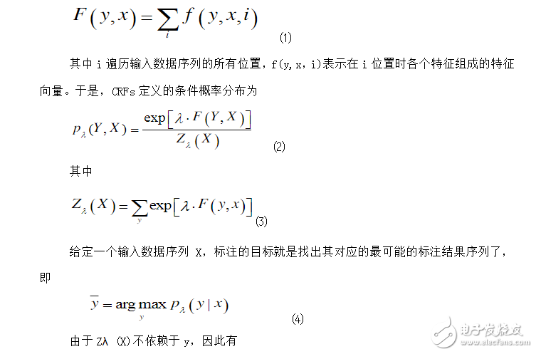
The parameter estimation of the CRFs model is usually implemented by the L-BFGS algorithm. The CRFs decoding process, which is the process of solving the unknown string annotation, requires a search to calculate a maximum joint probability on the string. The decoding process is performed using the Viterbi algorithm. CRFs have strong reasoning ability, can fully utilize context information as a feature, and can also add other external features arbitrarily, so that the information that the model can obtain is very rich. CRFs effectively solve other non-generated directed graph models by using only one exponential model as the joint probability of the entire marker sequence under the given observation sequence conditions, so that different feature weights in different states of the model can alternate with each other. The resulting problem of label offsets. These characteristics make CRFs theoretically suitable for Chinese part-of-speech tagging.
to sum upFirst of all, CRF, HMM (Hidden Horse Model) are often used to do the modeling of sequence annotation, like part of speech tagging, True casing. However, one of the biggest shortcomings of the hidden horse model is that it cannot solve the characteristics of the context due to its output independence hypothesis, which limits the choice of features, and another method called maximum entropy hidden horse model solves this problem. The selection feature, but because it is normalized at each node, only the local optimal value can be found, and the label bias is also brought about, which is not found in the training corpus. The situation is all ignored, and the conditional random field solves the problem very well. He does not normalize at each node, but all features are globally normalized, so the global optimal value can be obtained. At present, open source tools for conditional random field training and decoding only support chained sequences, complex is not supported, and training time is long, but the effect is ok. The limitation of the maximum entropy hidden horse model is that it uses the trained local model to make global predictions. The optimal prediction sequence is simply a combination of the local maximum entropy model by the viterbi algorithm. Conditional random field, hidden horse model, and maximum entropy hidden horse model can be used to do the sequence labeling model. However, each has its own characteristics. The HMM model directly models the transition probability and performance probability, and the statistical co-occurrence probability. The maximum entropy hidden horse model establishes a joint probability for the transition probability and the performance probability, and the statistical probability is the conditional probability.
In the calculation of the global probability, when doing normalization, the distribution of the data in the global is considered, rather than just local normalization, thus solving the problem of mark offset in MEMM.
Asic Antminer Machine:Bitmain Antminer E9 (2.4Gh),Bitmain Antminer E3 (190Mh),Bitmain Antminer G2
The latest ETC Ethash Miner of asic antminer machine is Bitmain Antminer E9,it has 2.4gh/s hashrate,It's very profitable
ANTMINER is the world's leading digital currency mining machine manufacturer. Its brand ANTMINER has maintained a long-term technological and market dominance in the industry, with customers covering more than 100 countries and regions. The company has subsidiaries in China, the United States, Singapore, Malaysia, Kazakhstan and other places.
Bitmain Antminer has a unique computing power efficiency ratio technology to provide the global blockchain network with outstanding computing power infrastructure and solutions. Since its establishment in 2013, ANTMINER BTC mining machine single computing power has increased by three orders of magnitude, while computing power efficiency ratio has decreased by two orders of magnitude. Bitmain's vision is to make the digital world a better place for mankind.
Asic Antminer Machine,E9 Etc Miner,E9 Eth Miner,Antminer E9 Eth Miner,antminer ETC Miner
Shenzhen YLHM Technology Co., Ltd. , https://www.hkcryptominer.com