In the following article, we will discuss decision trees, clustering algorithms, and regressions, point out the differences between them, and find out how to choose the most appropriate model based on different cases.
Supervised learning vs unsupervised learningUnderstanding the basics of machine learning is how to classify the two categories of supervised learning and unsupervised learning, because any problem in machine learning problems is ultimately one of these two categories.
In the case of supervised learning, we have datasets that some algorithms use as input. The premise is that we already know what the correct output format should look like (assuming there is a relationship between input and output).
The regression and classification problems we see later fall into this category.
Unsupervised learning, on the other hand, applies to situations where we are uncertain or do not know what the correct output should look like. In fact, we need to derive from the data what the correct structure should look like. The clustering problem is the main representative of this class.
In order to make the above classification clearer, I will list some real-world problems and try to classify them accordingly.
Example 1
Suppose you are running a real estate company. Considering the characteristics of the new house, you want to predict the sales price of this house based on the sales of other houses recorded before. The input dataset contains features of multiple houses, such as the number and size of bathrooms, and the variables you want to predict, often referred to as target variables, are prices in this example. Because I already know the selling price of the house in the data set, this is a question of supervised learning. To be more specific, this is a question about return.
Example 2
Suppose you did an experiment to infer whether someone would develop myopia based on certain physical measurements and genetic factors. In this case, the input data set is composed of human medical features, and the target variables are twofold: 1 indicates those who may develop myopia, and 0 indicates those who are not myopia. Since the values ​​of the target variables of the participants are known in advance (ie you already know if they are myopia), this is another question of supervised learning - more specifically, this is a classification problem.
Example 3
Suppose the company you are responsible for has a lot of customers. Based on their recent interactions with the company, recently purchased products, and their demographics, you want to group similar customers into groups and treat them in different ways—such as giving them exclusive discount coupons. In this case, some of the features mentioned above will be used as input to the algorithm, and the algorithm will determine the number or type of customers that should be. This is the most typical example of unsupervised learning, because we don't know what the output should look like in advance.
Having said that, now is the time to fulfill my promise, to introduce some more specific algorithms...
returnFirst, regression is not a single supervised learning technique, but the entire category to which many technologies belong.
The main idea of ​​regression is to give some input variables, we want to predict what the value of the target variable is. In the case of regression, the target variable is continuous - this means that it can take any value within the specified range. On the other hand, input variables can be either discrete or continuous.
Among the regression techniques, the most widely known are linear regression and logistic regression. Let us study the research carefully.
Linear regressionIn linear regression, we try to establish the relationship between the input variable and the target variable, which is represented by a straight line, usually called the regression line.
For example, suppose we have two input variables X1 and X2 and a target variable Y. This relationship can be expressed mathematically:
Y = a * X1 + b*X2 +c
Assuming that the values ​​of X1 and X2 have been provided, our goal is to adjust the three parameters a, b, and c so that Y is as close as possible to the actual value.
Take a moment to talk about an example!
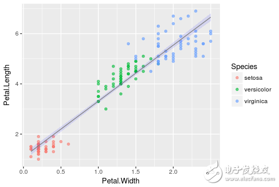
Suppose we already have an Iris dataset that already contains data on the size of the bracts and petals of different types of flowers, such as Setosa, Versicolor, and Virginica.
Using the R software, assuming that the width and length of the petals have been provided, we need to implement a linear regression to predict the length of the sepals.
In mathematics, we will get the values ​​of a and b by the following relationship:
SepalLength = a * PetalWidth + b* PetalLength +c
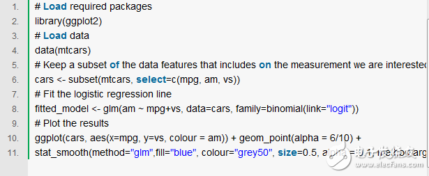
The corresponding code is as follows:

The results of the linear regression are shown in the figure below. The black dots indicate that the initial data points fit the regression line on the blue line, so the estimation results are obtained, a = -0.31955, b = 0.54178, and c = 4.19058. This result may be closest to the actual The situation is the length of the flowerbed.
From now on, by applying the values ​​of petal length and petal width to the defined linear relationship, we can also predict the length of the new data point.
The main idea here is exactly the same as linear regression. The biggest difference is that the regression line is no longer straight.
Instead, the mathematical relationship we are trying to establish is similar to the following form:
Y=g(a*X1+b*X2)
Here g() is a logical function.
Due to the nature of the logisTIc function, Y is continuous, in the range [0,1], can be understood as the probability of occurrence of an event.
I know that you like the example, so I will show you one more!
This time, we will experiment with the mtcars dataset, which includes 10 aspects of fuel consumption and vehicle design, and the performance of 32 cars produced in 1973-1974.
Using R, we will predict the probability of an automatic transmission (am = 0) or a manual (am = 1) car based on measurements of the V/S and Miles/(US) gallons.
Am = g(a * mpg + b* vs +c):
The results are shown below, where the black dots represent the initial points of the data set and the blue lines represent the fitted logistic regression lines for a = 0.5359, b = - 2.7957, and c = - 9.9183.
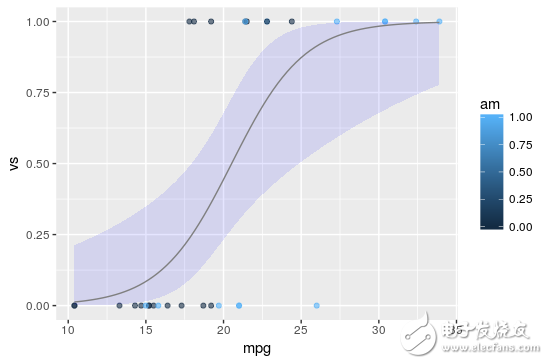
As mentioned earlier, we can observe that due to the form of the regression line, the logisTIc regression output value is only in the range [0, 1].
For any new car based on the V/S and Miles/(US) gallons, we can now predict the probability of the car's automatic transmission.
Decision treeThe decision tree is the second machine learning algorithm we will study. The decision tree eventually splits into regression and classification trees, so it can be used for supervised learning problems.
Admittedly, decision trees are one of the most intuitive algorithms that mimic the way people decide in most situations. What they do is basically to draw a "map" of all possible paths and draw the corresponding results in each case.
Graphical representations will help to better understand what we are discussing.
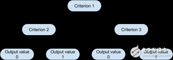
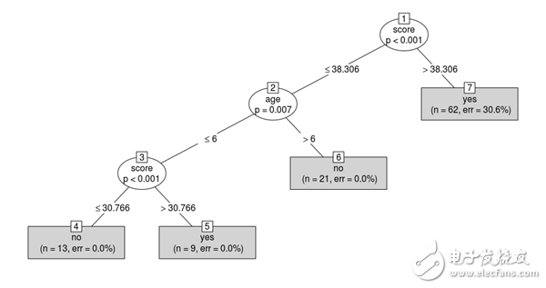
Based on such a tree, the algorithm can decide which path to follow in each step based on the corresponding standard value. The way the algorithm selects the partitioning criteria and the corresponding threshold for each level depends on the amount of information that the candidate variable has on the target variable and which setting minimizes the resulting prediction error.
Here is another example!
The data set discussed this time is readingSkills. It includes the student's test scores and scores.
We will classify students into native English speakers (naTIveSpeaker = 1) or foreigners (naTIveSpeaker = 0) based on a variety of metrics, including their score in the test, their shoe size, and their age.
For the implementation in R, we first need to install the party package.
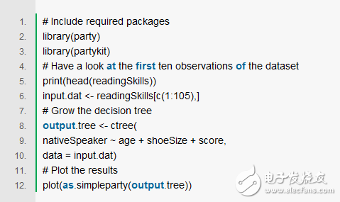
We can see that the first split criterion used is the score because it is very important when predicting the target variable, and the size of the shoe is not taken into account because it does not provide any useful information about the language.
Now, if we have a new student and know their age and score, we can predict if they are an English-speaking person!
Clustering AlgorithmSo far, we have only discussed some issues related to supervised learning. Now, we continue to study clustering algorithms, which are a subset of unsupervised learning methods.
So, just a little modification...
For clusters, if there is some initial data to dominate, we want to form a group, so that the data points of some groups are similar and different from the data points of other groups.
The algorithm we are going to learn is called k-means, and k is the number of clusters produced. This is one of the most popular clustering methods.
Remember the Iris dataset we used before? We will use it again.
For the sake of research, we used the petal measurement method to plot all the data points of the data set, as shown in the following figure:
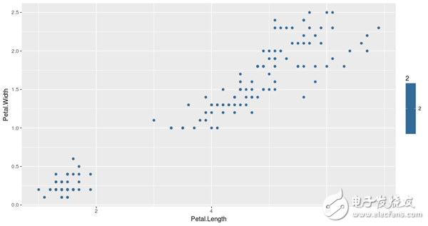
Based on the petal metrics, we will use the 3-means clustering method to aggregate the data points into 3 groups.
So how does 3-means, or k-means, work? The whole process can be summarized in a few simple steps:
Initialization step: For k = 3 clusters, the algorithm randomly selects 3 points as the center point of each cluster.
Cluster allocation step: The algorithm passes the remaining data points and assigns each data point to the nearest cluster.
Centroid move step: After cluster allocation, the center point of each cluster moves to the average of all points belonging to the cluster.
Steps 2 and 3 are repeated multiple times until there are no changes to the cluster assignment. The implementation of the k-means algorithm in R is very simple and can be implemented with the following code:
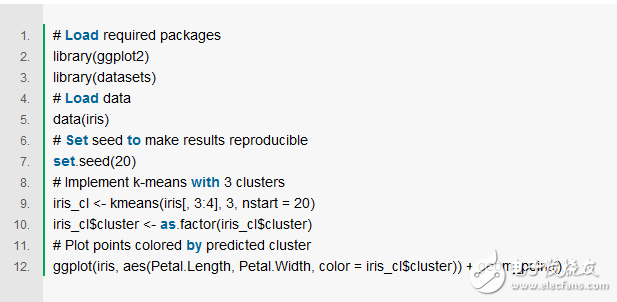
As can be seen from the results, the algorithm divides the data into three groups, each represented by three different colors. We can also observe that these clusters are formed according to the size of the petals. More specifically, red indicates a small flower petal, green indicates a relatively large petal, and blue indicates a medium-sized petal.
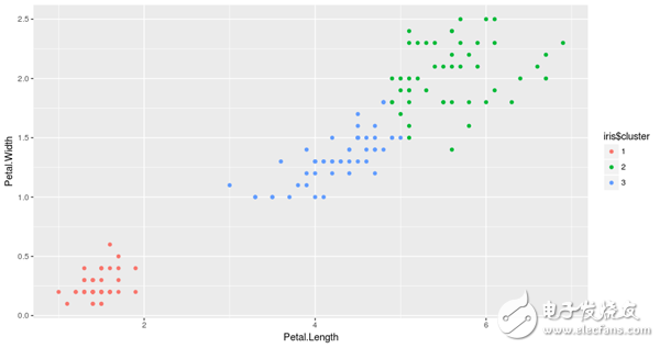
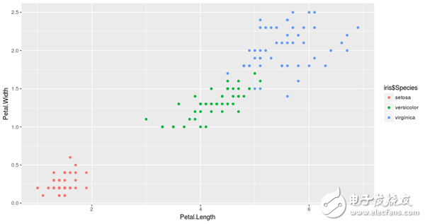
It is worth noting that in any cluster, the interpretation of the formation of the group requires some expert knowledge in the field. In our case, if you are not a botanist, you may not realize that what k-means does is to aggregate the iris into their different types, such as Setosa, Versicolor, and Virginica, without any knowledge about them. !
So if we draw the data again, this time is colored by their species, we will see the similarities in the cluster.
We have gone a long way from the beginning. We discussed regression (linear and logical) and decision trees, and finally discussed the k-means cluster. We also implemented some simple but powerful methods in R.
So what are the advantages of each algorithm? Which one should you choose in real life?
First of all, the methods presented are not some of the inapplicable algorithms - they are widely used in production systems around the world, so they need to be chosen according to different tasks, and choosing the right words can be quite powerful.
Secondly, in order to answer the above questions, you must be clear about what the advantages you are saying, because each method exhibits different advantages in different environments, such as interpretability, robustness, calculation time, and so on.
Cat 6 Lan Cable,Cat6 Ethernet Cable,Outdoor Cat6 Cable,Lan Cable Cat6
Zhejiang Wanma Tianyi Communication Wire & Cable Co., Ltd. , https://www.zjwmty.com